XGBoost vs LSTM: A Comparative Analysis of Time Series Forecasting for Stock Price Prediction
XGBoost and LSTM. Both are compelling in their own right, but which one is better? Let’s break it down in a friendly way!
Predicting stock / forex prices has always been the “holy grail” of finance. The market is influenced by countless factors, and its inherent volatility makes prediction a challenging task. Two popular models in this regard are XGBoost, a gradient boosting algorithm, and LSTM, a type of recurrent neural network. Both have their strengths and weaknesses, and today, we’ll compare the math and mechanics behind each.
XGBoost (Extreme Gradient Boosting)
What is it?
XGBoost stands for eXtreme Gradient Boosting. It’s a boosting algorithm, primarily used for regression and classification problems. In our case, we’re looking at regression—predicting a continuous value (like stock prices) .Let’s unpack it some more:
1. Boosting:
Before we get too deep into XGBoost, let’s understand what boosting is. Boosting is a machine learning ensemble meta-algorithm to reduce bias and variance in supervised learning. The idea is simple: instead of relying on one model, why not create a series of models (each correcting the errors of the previous one) and then combine their outputs?
2. Tree Boosting:
XGBoost primarily uses decision trees as its weak learners. A decision tree is like a flowchart that helps make a decision based on answering a series of questions. The beauty of XGBoost is how it uses these trees.
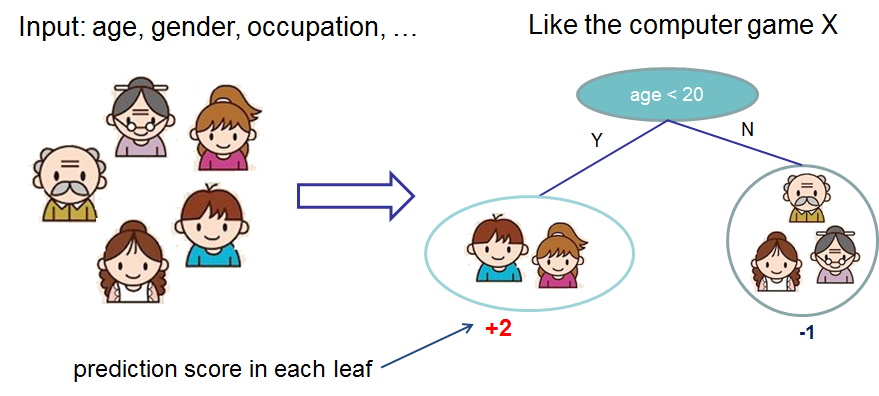
Each time a tree is added, it’s fit on the residual errors of the whole ensemble. This means the new tree tries to correct the mistakes made by the previous trees.
3. Regularization:
Regularization is one of the features that makes XGBoost stand out. While standard boosting algorithms just focus on reducing the loss (i.e., the difference between the predicted and actual values), XGBoost also focuses on keeping the model simple.
The objective function in XGBoost is given by:
$$ \text{Obj}(\theta) = L(\theta) + \Omega(\theta) $$
Where:
- $ L(\theta) $ is the loss function.
- $ \Omega(\theta) $ is the regularization term.
The regularization term penalizes complex models, which helps in reducing overfitting.
4. Handling Missing Data:
Real-world data is messy. Missing values are a common problem. XGBoost can naturally handle missing data. When it encounters a missing value at a node, it tries both the left and right child and learns the best direction to go during training. This is a significant advantage over other algorithms.
5. Parallel and Distributed Computing:
One reason XGBoost is so popular is its scalability. The algorithm is designed to be parallelized. While tree algorithms are usually hard to parallelize (since each step depends on the previous), XGBoost tackles this by creating a system where trees can be built in parallel.
6. Flexibility:
XGBoost supports regression, classification, ranking, and user-defined prediction tasks. It works with NumPy arrays, Pandas dataframes, SQL tables, and other data types. Plus, it provides several hyperparameters for fine-tuning and improving the model’s performance.
Now, let’s look at code examples for XGBoost run it, and see how it performs.
   import numpy as np
   import matplotlib.pyplot as plt
   from pandas_datareader import data as pdr
   import yfinance as yf
   from xgboost import XGBRegressor
   from sklearn.metrics import mean_squared_error
   from math import sqrt
   from sklearn.preprocessing import MinMaxScaler

   # Configure Yahoo Finance data source
   yf.pdr_override()

   # Download historical stock data
   ticker = "AAPL"
   start_date = "2015-01-01"
   end_date = "2023-01-01"
   stock_data = pdr.get_data_yahoo(ticker, start=start_date, end=end_date)

   # Normalize the dataset
   scaler = MinMaxScaler(feature_range=(0, 1))
   scaled_close = scaler.fit_transform(stock_data["Close"].values.reshape(-1, 1))

   # Create a dataset with lagged values as features
   def create_dataset(data, lag=1):
       X, y = [], []
       for i in range(len(data) - lag - 1):
           X.append(data[i:(i + lag), 0])
           y.append(data[i + lag, 0])
       return np.array(X), np.array(y)

   lag = 5
   X, y = create_dataset(scaled_close, lag)

   # Split the data into training and testing sets
   train_size = int(len(X) * 0.8)
   X_train, X_test = X[:train_size], X[train_size:]
   y_train, y_test = y[:train_size], y[train_size:]

   # Train the XGBRegressor model
   model = XGBRegressor(objective='reg:squarederror',
                        n_estimators=100,
                        tree_method='auto',
                        )
   model.fit(X_train, y_train)

   # Make predictions
   predicted_stock_price = model.predict(X_test)
   predicted_stock_price = scaler.inverse_transform(predicted_stock_price.reshape(-1, 1))

   # De-normalize the test data
   real_stock_price = scaler.inverse_transform(y_test.reshape(-1, 1))

   # Calculate the root mean squared error (RMSE)
   rmse = sqrt(mean_squared_error(real_stock_price, predicted_stock_price))
   print("RMSE: ", rmse)

   # Plot the actual vs. predicted closing prices
   plt.figure(figsize=(12, 6))
   plt.plot(stock_data["Close"].index[:train_size + lag], stock_data["Close"][:train_size + lag], label="Training data")
   plt.plot(stock_data["Close"].index[train_size + lag:train_size + lag + len(predicted_stock_price)], stock_data["Close"][train_size + lag:train_size + lag + len(predicted_stock_price)], label="Actual closing prices")
   plt.plot(stock_data["Close"].index[train_size + lag:train_size + lag + len(predicted_stock_price)], predicted_stock_price, label="Predicted closing prices")
   plt.xlabel("Date")
   plt.ylabel("Closing Price")
   plt.title(f"{ticker} Stock Closing Price Prediction using XGBRegressor")
   plt.legend()
   plt.show()
The Root Mean Square Error (RMSE) is a measure of the differences between values predicted by a model and the values observed. It provides a way to see how well the model’s predictions match the actual data. The smaller the RMSE, the better the model’s predictions match the observed data.
In our case, an RMSE of 22.0776 means that, on average, the model’s predictions are off by about 22.08 dollars from the actual closing prices of the AAPL stock over the test period. This gives you an idea of the magnitude of error we might expect when using this model to make predictions on new data.
Although the RMSE is a good measure of how well the model performs, it doesn’t tell us if the model is biased or
unbiased or if we’re overfitting / underfitting the data. To get a better idea of how the model is performing, we should
backtest it agaist RT data and see how it performs.
One can enhance the model by tuning the hyperparameters. For example, we can try changing the number of trees in the
ensemble, the maximum depth of each tree, and the learning rate using optuna to find the best hyperparameters.

To interpret this further:
If the stock prices range from, say, 100 dollars to 500 dollars, then an RMSE of 22.08 might be considered relatively small. If the stock prices range from, say, 20 dollars to 50 dollars, then an RMSE of 22.08 would be considered large. So, the value of RMSE should be interpreted in the context of the range and scale of the data you’re working with.
Takeaway:
Imagine you’re teaching a kid to ride a bike. Every time the kid makes a mistake, you correct it, ensuring the same mistake isn’t repeated. This iterative correction process is similar to how XGBoost builds its trees.
Furthermore, just like how you wouldn’t want the kid to focus only on one way of pedaling (because they might become too rigid and fall over), XGBoost uses regularization to ensure its model doesn’t get too focused on the training data and lose its generalization power.
In essence, XGBoost is like a smart, adaptive, and disciplined approach to learning from data and making predictions. It’s not just about learning; it’s about learning the right way!
Now that we’ve covered XGBoost, let’s look at LSTM.
LSTM (Long Short-Term Memory)
What is it?
LSTMs were introduced to combat the long-term dependency problem of traditional RNNs, which are exploding/vanishing gradients. In simpler terms, while RNNs are great at understanding sequences, they falter when the sequences are too long. LSTMs, with their unique structure, can remember and retrieve information over long periods, making them a popular choice for time series forecasting, natural language processing, and more.

A Closer Look at the Components:
-
Cell State: Often visualized as a horizontal line running through the LSTM unit, this is the “memory” of the LSTM. It stores information on what the LSTM has seen in the sequence so far. Its magic lies in its ability to retain or forget information, making it adept at handling long sequences.
-
Gates: These are a series of neural network layers that regulate the flow of information into and out of the cell state.
-
Forget Gate: This gate decides what information from the cell state should be thrown away or kept. It looks at the previous hidden state and the current input and outputs a number between 0 (forget) and 1 (keep) for each number in the cell state.
$$f_t = \sigma(W_f \cdot [h_{t-1}, x_t] + b_f)$$
-
Input Gate: This gate updates the cell state with new information. It has two parts:
- A sigmoid layer that decides which values to update.
- A tanh layer that creates a vector of new candidate values.
$$i_t = \sigma(W_i \cdot [h_{t-1}, x_t] + b_i)$$ $$ C_t = \text{tanh}(W_C \cdot [h_{t-1}, x_t] + b_C)$$
-
Output Gate: This gate decides what the next hidden state should be. It looks at the previous hidden state and the current input and outputs the hidden state based on the updated cell state.
$$ o_t = \sigma(W_o \cdot [h_{t-1}, x_t] + b_o)$$ $$h_t = o_t \times \text{tanh}(C_t)$$
-
Why All These Gates?
You can think of these gates as filters. In our daily lives, we constantly receive information, but not all of it is worth remembering. The gates in LSTMs help the network decide what’s crucial to remember, what’s okay to forget, and how to update the current knowledge based on new information.
Analogy:
Imagine reading a long story. Your brain doesn’t remember every single detail, like the color of the farmer’s shirt in chapter 3 (unless it’s vital to the plot). Instead, it captures the essence, the character development, and major events. When a later chapter references a past event, you recall it. This is similar to how LSTMs operate. The gates are like your cognitive filters, deciding what details to store, recall, or forget.
Applications of LSTM:
While we’re focused on stock price prediction here, LSTMs shine in various domains:
- Natural Language Processing: LSTMs are popular in tasks like sentiment analysis, machine translation, and text generation because of their ability to understand the context over long sentences.
- Music Generation: They can generate new music by understanding the patterns in sequences of notes.
- Video Analysis: LSTMs can be used to recognize actions in videos where understanding the sequence of frames is crucial.
   import numpy as np
   import matplotlib.pyplot as plt
   from pandas_datareader import data as pdr
   import yfinance as yf
   from sklearn.preprocessing import MinMaxScaler
   from sklearn.metrics import mean_squared_error
   from math import sqrt
   from keras.models import Sequential
   from keras.layers import Dense, LSTM, Dropout
   from keras.callbacks import EarlyStopping
   # Configure Yahoo Finance data source
   yf.pdr_override()

   # Download historical stock data
   ticker = "AAPL"
   start_date = "2015-01-01"
   end_date = "2023-01-01"
   stock_data = pdr.get_data_yahoo(ticker, start=start_date, end=end_date)

   # Normalize the dataset
   scaler = MinMaxScaler(feature_range=(0, 1))
   scaled_data = scaler.fit_transform(stock_data["Close"].values.reshape(-1, 1))


   # Create a dataset with lagged values as features
   def create_dataset(data, lag=1):
       X, y = [], []
       for i in range(len(data) - lag - 1):
           X.append(data[i:(i + lag)])
           y.append(data[i + lag])
       return np.array(X), np.array(y)


   lag = 3
   X, y = create_dataset(scaled_data, lag)

   # Reshape input to be [samples, timesteps, features]
   X = np.reshape(X, (X.shape[0], X.shape[1], 1))

   # Split the data into training and testing sets
   train_size = int(len(X) * 0.8)
   X_train, X_test = X[:train_size], X[train_size:]
   y_train, y_test = y[:train_size], y[train_size:]

   # Define the LSTM model
   model = Sequential()
   model.add(LSTM(units=100, return_sequences=True, input_shape=(X_train.shape[1], 1), kernel_regularizer='l2',
                  recurrent_regularizer='l2'))
   model.add(Dropout(0.3))
   model.add(LSTM(units=100, kernel_regularizer='l2', recurrent_regularizer='l2'))
   model.add(Dropout(0.3))
   model.add(Dense(units=1))
   model.compile(optimizer='adam', loss='mean_squared_error')
   model.fit(X_train, y_train, epochs=100, batch_size=32, callbacks=[EarlyStopping(monitor='loss', patience=10)])

   # Make predictions
   predicted_stock_price = model.predict(X_test)
   predicted_stock_price = scaler.inverse_transform(predicted_stock_price)

   # De-normalize the test data
   real_stock_price = scaler.inverse_transform(y_test)

   # Calculate the root mean squared error (RMSE)
   rmse = sqrt(mean_squared_error(real_stock_price, predicted_stock_price))
   print("RMSE: ", rmse)

   # Plot the actual vs. predicted closing prices
   plt.figure(figsize=(12, 6))
   plt.plot(stock_data["Close"].index[:train_size + lag], stock_data["Close"][:train_size + lag], label="Training data")
   plt.plot(stock_data["Close"].index[train_size + lag + 1:], stock_data["Close"][train_size + lag + 1:],
   label = "Actual closing prices")
   plt.plot(stock_data["Close"].index[train_size + lag + 1:], predicted_stock_price, label="Predicted closing prices")
   plt.xlabel("Date")
   plt.ylabel("Closing Price")
   plt.title(f"{ticker} Stock Closing Price Prediction using LSTM")
   plt.legend()
   plt.show()
Interpreting LSTM Predictions

The RMSE value of 7.57 can be interpreted as the model’s predictions being off by about $7.57 on average from the actual closing prices of the AAPL stock over the test period.
Just as with the XGBoost model, it’s essential to view the RMSE in context:
If the stock prices range from 100 dollars to 500 dollars, an RMSE of 7.57 can be considered relatively small. Conversely, if stock prices are between 20 dollars and 50 dollars, an RMSE of 7.57 would be deemed significant.

While RMSE provides a straightforward measure of a model’s prediction error magnitude, it doesn’t paint a complete picture of the model’s quality or appropriateness for a given task. To get a comprehensive understanding of model performance, it’s essential to use a combination of metrics and visual assessments. By doing so, you can ensure a more robust and reliable model evaluation process. Here are some of the metrics and methods that can be employed alongside RMSE:
- Mean Absolute Error (MAE): MAE calculates the average of the absolute errors between the predicted and the actual values. Unlike RMSE, MAE is less sensitive to outliers since it doesn’t square the errors.
$$ \text{MAE} = \frac{1}{n} \sum_{i=1}^{n} |y_i - \hat{y}_i| $$
- Mean Bias Deviation (MBD): This metric calculates the average bias in the predictions. It can show if the model consistently overestimates or underestimates the target variable.
$$ \text{MBD} = \frac{\sum_{i=1}^{n} (y_i - \hat{y}_i)}{n} $$
- Mean Absolute Percentage Error (MAPE): MAPE expresses the prediction errors as a percentage, making it scale-independent and easy to interpret. It’s especially useful when you want to understand the error relative to the actual values.
$$ \text{MAPE} = \frac{1}{n} \sum_{i=1}^{n} \left|\frac{y_i - \hat{y}_i}{y_i}\right| \times 100 $$
-
R-squared (Coefficient of Determination): R-squared measures the proportion of the variance in the dependent variable that is predictable from the independent variables. A value of 1 indicates perfect predictions, while a value of 0 means the model does no better than simply predicting the mean of the target variable.
-
Residual Plots: These are graphical representations that display the difference between the actual and predicted values. Patterns in residual plots can indicate issues like heteroscedasticity or model misspecification.

As you can see, the residuals are randomly scattered around the center line, indicating that the model is capturing the patterns in the data well. The range at some time periods indicates that the model’s predictions are, on average, off by an amount between -5 and 5 units from the actual values. In the context of stock prices, this means the predicted closing prices can be up 5 dollars too high or 5 dollars too low from the actual closing prices.
- Actual vs. Predicted Plots: By plotting the actual values against the predicted values like we did, you can visually assess how closely the model’s predictions align with the true outcomes.
Why This Architecture?
The architecture chosen here consists of two LSTM layers, with Dropout layers for regularization. The first LSTM layer, with 100 units, returns sequences to ensure a multi-layer stack of LSTMs, enhancing the model’s learning capability. Dropout layers, set at 0.3, reduce overfitting by randomly ignoring 30% of neurons during training. This architecture, combined with L2 regularization in the LSTM layers, strikes a balance between complexity and overfitting, making it suitable for capturing intricate patterns in the time series data of stock prices.
Visual Insights
Taking a glance at Figure 6, which showcases our LSTM predictions against the actual stock prices, offers further insight:
- Trend Analysis: Does the predicted stock price follow the general trend of the actual stock price? If the answer is yes, then our model is capturing the larger movements and patterns in the stock data.
- Volatility: Stock markets are inherently volatile. If our model can capture sudden spikes or drops, it’s a testament to its ability to react to market changes.
- Overfitting/Underfitting: If our predictions are too perfect, it’s a sign of overfitting. If they’re way off, then it’s possibly underfitting or not capturing the essential patterns.
Recommendations for Improvement
While an RMSE of 7.57 is a promising start, there’s always room for improvement in the world of machine learning:
- Feature Engineering: Incorporating more features, like trading volume, other technical indicators, or even external factors (like news sentiment), can improve the model’s accuracy.
- Hyperparameter Tuning: LSTMs come with various hyperparameters. Playing around with these (like the number of layers, the number of units in each layer, learning rate, etc.) can lead to better results.
- Ensembling: Combining the LSTM with other models, or using multiple LSTMs trained on different features, might help capture more patterns in the data.
Conclusion
In the pursuit of predicting stock prices, two models - XGBoost and LSTM - were examined. XGBoost, an ensemble boosting algorithm, iteratively corrects errors from its ensemble of decision trees. It stands out with features like regularization, handling missing data, and scalability. On the other hand, LSTM, a type of recurrent neural network, excels in understanding long sequences, making it a strong candidate for time series forecasting.
From my experiments, XGBoost yielded an RMSE of 22.0776, indicating predictions were off by about 22.08 dollars from the actual AAPL stock prices. LSTM showcased a more impressive performance with an RMSE of 7.57, suggesting deviations of roughly 7.57 dollars from real stock prices.
However, while these results provide a glimpse into each model’s capabilities, predicting stock prices remains a complex task due to so many influencing factors. Models can guide decisions, but they should be used in conjunction with comprehensive market analysis. Both XGBoost and LSTM have their strengths, and the choice between them should align with specific project needs and data characteristics.